Yes, it’s me. 能够在Oracle官方站点的ACE主页面作为Spotlight人物被介绍,很荣幸。Oracle的技术生涯可以用此做个注解了。
BTW, 上面那张ACE全家福的二排正中间也能找到我,2014年OOW期间的照片,应该是迄今为止中国ACE专家在旧金山会和最全的一届。

Yes, it’s me. 能够在Oracle官方站点的ACE主页面作为Spotlight人物被介绍,很荣幸。Oracle的技术生涯可以用此做个注解了。
BTW, 上面那张ACE全家福的二排正中间也能找到我,2014年OOW期间的照片,应该是迄今为止中国ACE专家在旧金山会和最全的一届。
##什么是Sharding
> Sharding is a data tier architecture in which data is horizontally partitioned across independent databases. Each database in such configuration is called a shard. All of the shards together make up a single logical database which is referred to as a sharded database or SDB.
Sharding是指数据层的水平分区,实际上在之前的Oracle版本中,分区已经是数据仓库系统非常常用的技术手段,但是在12.2之前,一个分区表的所有分区只能存储在一个数据库中,而在12.2之后,一个分区表的多个分区可以存储在不同的数据库里,这就被称为Sharding。为什么Sharding这么被大家期待?因为可能很多人都在说,Oracle的水平扩展能力不够强,虽然有RAC,但是集群节点越多内耗就越多,这样的水平扩展能力跟Hadoop之类的方案相比是不足的。我们先不评判这样的看法是不是正确,Oracle 12.2要告诉大家的是,要Sharding?要分库分表?要线性水平扩展?没问题,给你。
假设这样的分库分表一共跨了10个Oracle数据库,那么这10个Oracle数据库对于前端应用来说是透明的,是一个统一的逻辑数据库,称为一个sharded数据库,或者简称为一个SDB,而在这个SDB中每个数据库被称为一个shard。
一张大表可以根据规则被分割到每个shard中,在每个shard里拥有相同的字段结构,但是却拥有不同的数据,这样的一张表被称为sharded table。
##Sharding适合所有的数据库应用吗?
既然Sharding听上去很厉害,那么是不是现在只要遇到有性能问题的数据库,一律都可以使用Sharding技术来解决呢?当然不,Sharding不会也不可能是FAST=TRUE这样的参数。一个适合Sharding技术的应用,必须有非常好的数据模型,和清晰的数据分布策略(比如是一致性哈希,范围或者列表分区),并且访问这些数据也是总要通过shard key来过滤的,只有这样,才能在整个Sharded数据库架构中很好地将请求路由到合适的数据库上。这样的shard key可能会是客户编号,国家编号,身份证号码等。
##Sharding有哪些缺点?
在我们颂扬一项技术之前,先看一下这项技术会带来哪些不便,是更理智的做法,要知道世界上并无十全十美的事物。
在Wikipedia([https://en.wikipedia.org/wiki/Shard_(database_architecture)])中对于Shard的坏处有如下的定义。
> •Increased complexity of SQL – Increased bugs because the developers have to write more complicated SQL to handle sharding logic.
> •Sharding introduces complexity – The sharding software that partitions, balances, coordinates, and ensures integrity can fail.
> •Single point of failure – Corruption of one shard due to network/hardware/systems problems causes failure of the entire table.
> •Failover servers more complex – Failover servers must themselves have copies of the fleets of database shards.
> •Backups more complex – Database backups of the individual shards must be coordinated with the backups of the other shards.
> •Operational complexity added – Adding/removing indexes, adding/deleting columns, modifying the schema becomes much more difficult.
1. 增加了SQL的复杂性。因为开发人员必须要写更复杂的SQL来处理sharding的逻辑。
2. Sharding本身带来的复杂性。sharding软件需要照顾分区,数据平衡,访问协调,数据完整性。
3. 单点故障。一个shard损坏可能导致整张表不可访问。
4. 失效接管服务器也更复杂。因为负责失效接管的服务器必须拥有任何可能损坏的shard上的数据。
5. 备份也更复杂。多个shard可能都需要同时备份。
6. 维护也更复杂。比如增加删除索引,增减删除字段,修改表定义等等,都变得更困难。
庆幸的是,这上面的大部分缺点,在Oracle 12.2 Sharding中都无需担心。
##Oracle Sharding Architecture
跟那些NoSQL数据库架构不一样,Oracle Sharding在提供sharding的同时,并没有牺牲掉关系型数据库所带来的优秀特性,比如说关系型数据建模,SQL编程接口,丰富的数据类型,在线的表结构变更,充分利用CPU多核的扩展性,高级安全,压缩,高可用,ACID特征,一致读,所有的Oracle数据库的优势仍然还在那里,但是,额外,提供了sharding的优势。
对于Oracle Sharding的上层来说,使用的是Oracle GDS(Global Data Services)框架来实现自动部署和shading的管理以及拓扑复制。GDS还同时提供了对于整个SDB访问的负载均衡和基于位置的路由功能。在GDS框架中,global service manager负责将应用过来的请求转发到合适的shard上,另外还有一个shard catalog数据库,支持跨shard的查询功能,同时SDB的配置数据也都存在这个catalog数据库中。
对于Oracle Sharding的底层来说,使用的是Oracle长久以来一直存在的分区(partitioning)技术。Oracle Sharding就其本质上来说,实际上就是分布式分区,将以前的分区扩展支持到跨不同的物理数据库上。
因此创建一个sharded table的语法,跟以前创建一张分区表的语法也是非常相像的,以前称为分区键的字段现在被称为“sharding key”。
CREATE SHARDED TABLE customers
( cust_id NUMBER NOT NULL
, name VARCHAR2(50)
, address VARCHAR2(250)
, region VARCHAR2(20)
, class VARCHAR2(3)
, signup DATE
CONSTRAINT cust_pk PRIMARY KEY(cust_id) )
PARTITION BY CONSISTENT HASH (cust_id)
TABLESPACE SET ts1
PARTITIONS AUTO
;
在上面的语法中出现了一些新的关键字,比如“CONSISTENT HASH”,“TABLESPACE SET”,后面会详细解释。
Sharded table的每个分区是在表空间这个层面分布到不同的数据库(shard)中的,每个分区都必须在一个单独的表空间中。当使用consistent hash来进行分区以后,表空间会自动分布到不同的shard中,最终提供一个平均分布的数据架构。
除了consistent hash方式之外,Oracle还提供了基于range和list,和两层复合分区(range-consistent hash和list-consistent hash)的方式来进行Sharding,这对于熟悉Oracle分区技术的人来说一点儿也不陌生。
Oracle Sharding整合了Oracle很多成熟的技术,比如复制技术,Oracle Data Guard和Oracle Goldengate;比如高可用技术,Oracle RAC;比如连接池技术,connection pool;当然还有在12.1中新发的GDS框架。
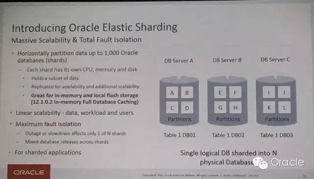
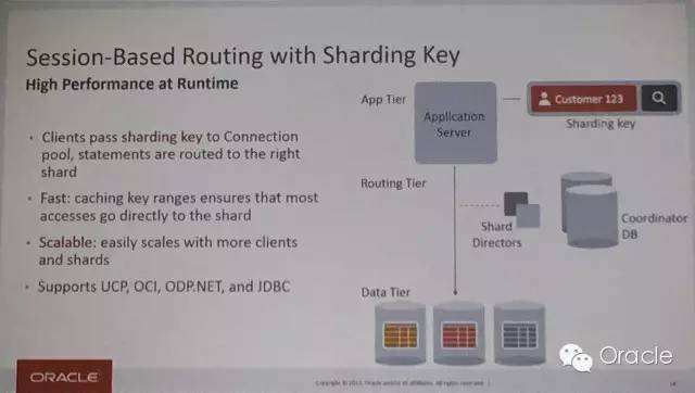
这个章节最后用2张PPT来结束,这是Eygel放出的在昨天旧金山OOW上Oracle介绍的Sharding技术的PPT。
_Oracle Sharding的实现_
_Sharding如何实现数据访问路由_
接下来的章节会继续介绍Oracle Sharding的详细实现和使用方法。
前几天PostgreSQL 9.5 Alpha 1版本刚刚发布,在新版本中吸引我注意的是BRIN index。为什么引人注意?因为这就是活脱脱的Oracle Exadata中的Storage Index和Oracle Database 12.1.0.2中的新功能Zone Maps。
Exadata的Storage Index不说了,因为那并非数据库范畴的解决方案,而Oracle数据库12.1.0.2中的新功能Zone Maps曾让我非常激动,但是最终发现该功能也只能在运行于Exadata上的Oracle中才能启用,略失望。
Zone Maps的解释如下:
Zone maps in an Oracle Database store minimum and maximum values of columns for a range of blocks (known as a zone). In addition to performing I/O pruning based on predicates of clustered fact tables, zone maps prune on predicates of dimension tables provided the fact tables are attribute-clustered by the dimension attributes though outer joins with the dimension tables.
BRIN index的解释如下:
BRIN stands for Block Range INdexes, and store metadata on a range of pages. At the moment this means the minimum and maximum values per block…So if a 10GB table of order contained rows that were generally in order of order date, a BRIN index on the order_date column would allow the majority of the table to be skipped rather than performing a full sequential scan.
同样的思路,在一个类索引结构中存储一定范围的数据块中某个列的最小和最大值,当查询语句中包含该列的过滤条件时,就会自动忽略那些肯定不包含符合条件的列值的数据块,从而减少IO读取量,提升查询速度。
以下借用Pg wiki中的例子解释BRIN indexes的强大。
 -- 创建测试表orders
 CREATE TABLE orders (
     id int,
     order_date timestamptz,
     item text);

 -- 在表中插入大量记录,Pg的函数generate_series非常好用。
 INSERT INTO orders (order_date, item)
 SELECT x, 'dfiojdso'
 FROM generate_series('2000-01-01 00:00:00'::timestamptz, '2015-03-01 00:00:00'::timestamptz,'2 seconds'::interval) a(x);

 -- 该表目前有13GB大小,算是大表了。
 # \dt+ orders
                    List of relations
  Schema |  Name  | Type  | Owner | Size  | Description
 --------+--------+-------+-------+-------+-------------
  public | orders | table | thom  | 13 GB |
 (1 row)

 -- 以全表扫描的方式查询两天内的记录,注意这里预计需要30s,这是一个存储在SSD上Pg数据库,因此速度已经很理想了。
 # EXPLAIN ANALYSE SELECT count(*) FROM orders WHERE order_date BETWEEN '2012-01-04 09:00:00' and '2014-01-04 14:30:00';
                                                                          QUERY PLAN
 -------------------------------------------------------------------------------------------------------------------------------------------------------------
  Aggregate  (cost=5425021.80..5425021.81 rows=1 width=0) (actual time=30172.428..30172.429 rows=1 loops=1)
    ->  Seq Scan on orders  (cost=0.00..5347754.00 rows=30907121 width=0) (actual time=6050.015..28552.976 rows=31589101 loops=1)
          Filter: ((order_date >= '2012-01-04 09:00:00+00'::timestamp with time zone) AND (order_date <= '2014-01-04 14:30:00+00'::timestamp with time zone))
          Rows Removed by Filter: 207652500
  Planning time: 0.140 ms
  Execution time: 30172.482 ms
 (6 rows)

 -- 接下来在order_date列上创建一个BRIN index
 CREATE INDEX idx_order_date_brin
   ON orders
   USING BRIN (order_date);

 -- 查看这个BRIN index占多少物理空间,13GB的表,而BRIN index只有504KB大小,非常精简。
 # \di+ idx_order_date_brin
                               List of relations
  Schema |        Name         | Type  | Owner | Table  |  Size  | Description
 --------+---------------------+-------+-------+--------+--------+-------------
  public | idx_order_date_brin | index | thom  | orders | 504 kB |
 (1 row)

 -- 再次执行相同的SQL,看看性能提升多少。速度上升到只需要6秒钟,提升了5倍。如果这是存储在HDD上的Pg库,这个效果还能更明显。
 # EXPLAIN ANALYSE SELECT count(*) FROM orders WHERE order_date BETWEEN '2012-01-04 09:00:00' and '2014-01-04 14:30:00';
                                                                               QUERY PLAN
 -----------------------------------------------------------------------------------------------------------------------------------------------------------------------
  Aggregate  (cost=2616868.60..2616868.61 rows=1 width=0) (actual time=6347.651..6347.651 rows=1 loops=1)
    ->  Bitmap Heap Scan on orders  (cost=316863.99..2539600.80 rows=30907121 width=0) (actual time=36.366..4686.634 rows=31589101 loops=1)
          Recheck Cond: ((order_date >= '2012-01-04 09:00:00+00'::timestamp with time zone) AND (order_date <= '2014-01-04 14:30:00+00'::timestamp with time zone))
          Rows Removed by Index Recheck: 6419
          Heap Blocks: lossy=232320
          ->  Bitmap Index Scan on idx_order_date_brin  (cost=0.00..309137.21 rows=30907121 width=0) (actual time=35.567..35.567 rows=2323200 loops=1)
                Index Cond: ((order_date >= '2012-01-04 09:00:00+00'::timestamp with time zone) AND (order_date <= '2014-01-04 14:30:00+00'::timestamp with time zone))
  Planning time: 0.108 ms
  Execution time: 6347.701 ms
 (9 rows)

 --能够让用户自行设定一个range中可以包含的数据块数,也是很体贴的设计。默认情况下一个range包含128个page,我们可以修改为更小或者更大,包含的page越少则精度越细,相应的BRIN index也就会越大;反之则精度粗,BRIN index小。
 -- 创建一个每个range包含32 pages的索引。
 CREATE INDEX idx_order_date_brin_32
 ON orders
 USING BRIN (order_date) WITH (pages_per_range = 32);

 -- 再创建一个每个range包含512 pages的索引。
 CREATE INDEX idx_order_date_brin_512
 ON orders
 USING BRIN (order_date) WITH (pages_per_range = 512);

--比较一下各个索引的大小。
 # \di+ idx_order_date_brin*
                                  List of relations
  Schema |          Name           | Type  | Owner | Table  |  Size   | Description
 --------+-------------------------+-------+-------+--------+---------+-------------
  public | idx_order_date_brin     | index | thom  | orders | 504 kB  |
  public | idx_order_date_brin_32  | index | thom  | orders | 1872 kB |
  public | idx_order_date_brin_512 | index | thom  | orders | 152 kB  |
 (3 rows)
延展阅读:
Postgres 9.5 feature highlight: BRIN indexes
WAITING FOR 9.5 – BRIN: BLOCK RANGE INDEXES